Covariate Balance Diagnostics in Causal Inference

⚖️ Covariate Balance Diagnostics

Ensuring that covariates are balanced across treatment groups is critical for reducing bias in causal inference. Diagnostics help verify whether matching or weighting strategies have achieved this.

---

1. 🧪 Simulate Confounded Data

set.seed(123)
n <- 1000

X1 <- rnorm(n)
X2 <- rbinom(n, 1, 0.5)
logit_p <- -0.5 + 0.7 * X1 + 1.2 * X2
p_treat <- 1 / (1 + exp(-logit_p))
W <- rbinom(n, 1, p_treat)

Y <- 3 * W + 0.5 * X1 + 0.8 * X2 + rnorm(n)
data <- data.frame(X1, X2, W, Y)

---

2. 🎯 Perform Propensity Score Matching

match_model <- matchit(W ~ X1 + X2, data = data, method = "nearest", distance = "logit")
summary(match_model)

## 
## Call:
## matchit(formula = W ~ X1 + X2, data = data, method = "nearest", 
##     distance = "logit")
## 
## Summary of Balance for All Data:
##          Means Treated Means Control Std. Mean Diff. Var. Ratio eCDF Mean
## distance        0.6128        0.4582          0.8838     0.8746    0.2245
## X1              0.2922       -0.3106          0.6420     0.9700    0.1739
## X2              0.6125        0.3537          0.5313          .    0.2588
##          eCDF Max
## distance   0.3342
## X1         0.2779
## X2         0.2588
## 
## Summary of Balance for Matched Data:
##          Means Treated Means Control Std. Mean Diff. Var. Ratio eCDF Mean
## distance        0.6643        0.4582          1.1782     0.5242    0.3023
## X1              0.4617       -0.3106          0.8225     0.8641    0.2261
## X2              0.7096        0.3537          0.7305          .    0.3559
##          eCDF Max Std. Pair Dist.
## distance   0.4803          1.1782
## X1         0.3865          1.0319
## X2         0.3559          0.8829
## 
## Sample Sizes:
##           Control Treated
## All           458     542
## Matched       458     458
## Unmatched       0      84
## Discarded       0       0

---

3. 📊 Balance Diagnostics with cobalt

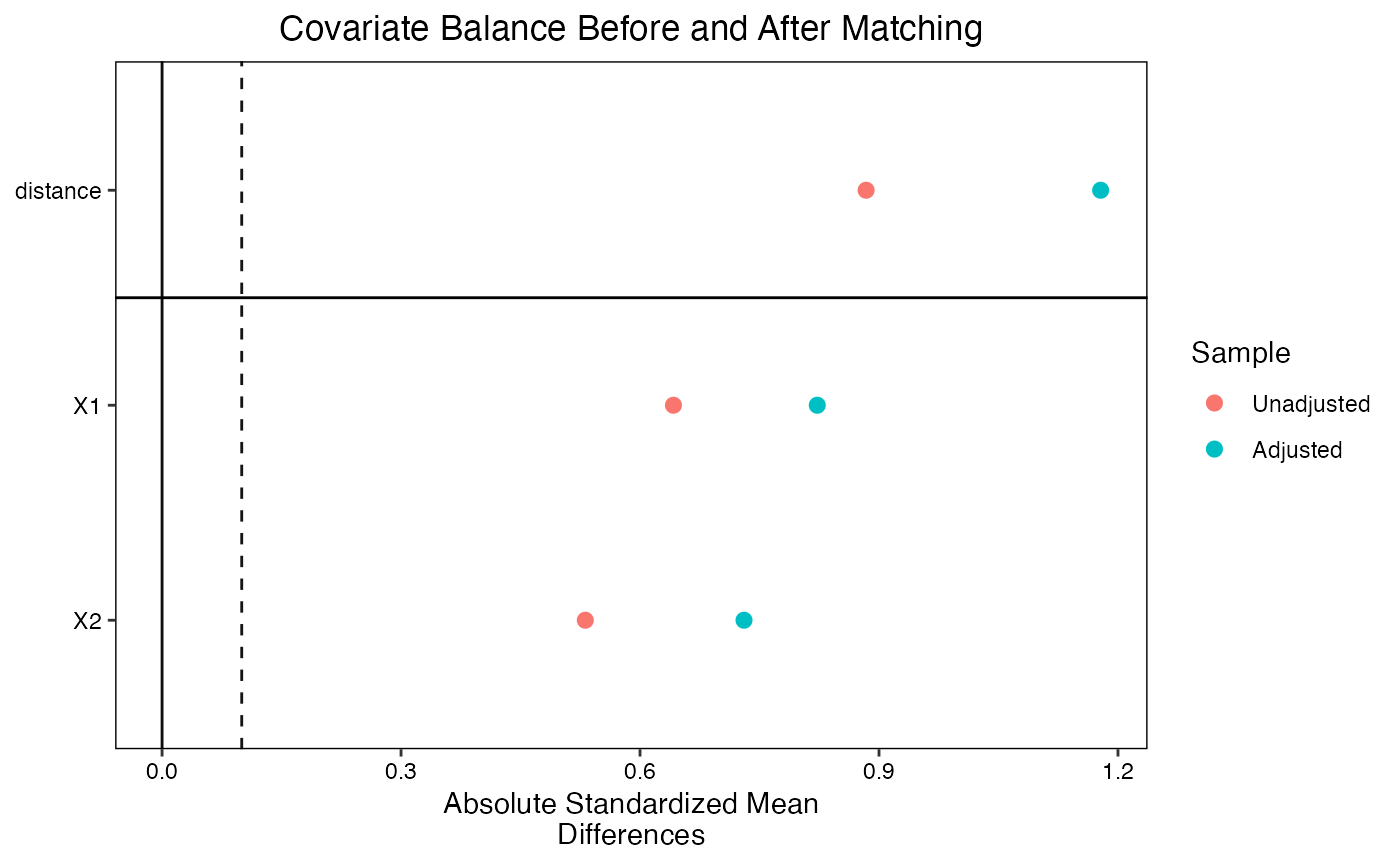
love.plot(match_model, binary = "std", var.order = "unadjusted",
          abs = TRUE, thresholds = c(m = .1),
          title = "Covariate Balance Before and After Matching")

---

4. ✅ Interpreting Balance Metrics

• Standardized Mean Differences (SMD): < 0.1 considered balanced
• Look for reduction in SMD after matching
• Avoid overfitting and extreme weights

---

📖 References

• Austin (2009). Balance diagnostics for comparing the distribution of baseline covariates using standardized differences
• Stuart (2010). Matching Methods for Causal Inference: A Review and a Look Forward